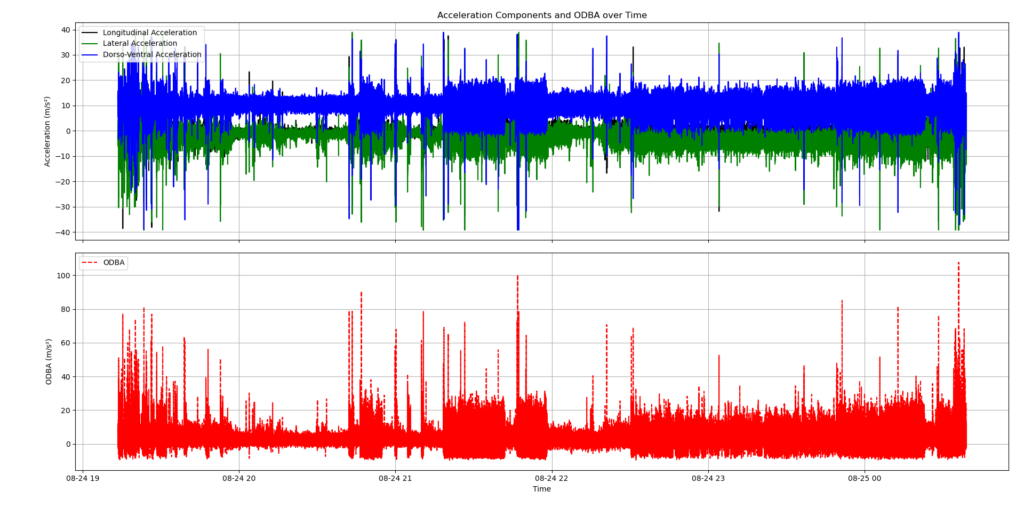
(time, acceleration_longitudinal,acceleration_lateral,acceleration_dorso_ventral) を含むデータ(data.csv)*読み込み、以下のような3軸の加速度の生波形とそれを元に計算したODBAの時系列グラフを表示します。
*BiPでOpenデータとなっているKatsufumi Sato (Atmosphere and Ocean Research Institute, University of Tokyo) 提供のオオミズナギドリのデータ (title: 9B41870_TS-AxyTrek_Movebank_YNo.6_release20210824) の一部を使用しています。
以下のPythonコード(plot_Acc.py)をテキストエディタで開き、JupyterLiteのノートブックにコピーして実行(右▼をクリック)します。
import pandas as pd
import matplotlib.pyplot as plt

# CSVファイルの読み込み
data = pd.read_csv('data.csv')

# 日時情報をpandasのdatetime型に変換(NaTを除外するためにエラー処理を追加)
data['time'] = pd.to_datetime(data['time'], errors='coerce')

# NaTを含む行を削除
data = data.dropna(subset=['time'])

# ODBAの計算
data['ODBA'] = (
    data['acceleration_longitudinal'].abs() +
    data['acceleration_lateral'].abs() +
    data['acceleration_dorso_ventral'].abs() - 9.8
)

# グラフの作成
fig, (ax1, ax2) = plt.subplots(2, 1, sharex=True, figsize=(10, 8))

# 加速度のプロット(上側のサブプロット)
ax1.plot(data['time'], data['acceleration_longitudinal'], color='black', label='Longitudinal Acceleration')
ax1.plot(data['time'], data['acceleration_lateral'], color='green', label='Lateral Acceleration')
ax1.plot(data['time'], data['acceleration_dorso_ventral'], color='blue', label='Dorso-Ventral Acceleration')
ax1.set_ylabel('Acceleration (m/s²)')
ax1.set_title('Acceleration Components and ODBA over Time')
ax1.grid(True)
ax1.legend(loc='upper left')

# ODBAのプロット(下側のサブプロット)
ax2.plot(data['time'], data['ODBA'], color='red', label='ODBA', linestyle='--')
ax2.set_ylabel('ODBA (m/s²)')
ax2.set_xlabel('Time')
ax2.grid(True)
ax2.legend(loc='upper left')

# グラフの保存
plt.tight_layout()
plt.savefig("output_graph.png", dpi=300, bbox_inches='tight')  # 画像として保存
plt.show()
出力された図は”output_graph.png”という名前でJupyterLite内で保存されているので、ダウンロードしてご利用ください。